Memory Profiling Part 5. Data Locality and Reuse Distances

Subscribe to my newsletter, support me on Patreon or by PayPal donation.

• Part 1: Introduction.
• Part 2: Memory Usage Case Study.
• Part 3: Memory Footprint with SDE.
• Part 4: Memory Footprint Case Study.
• Part 5: Data Locality and Reuse Distances (this article).

Data Locality and Reuse Distances

As you have seen from the previous case studies, there is a lot of information you can extract using modern memory profiling tools. Still, there are limitations which we will discuss next.

Consider memory footprint charts, shown in Figure 7 (in part 4). Such charts tell us how many bytes were accessed during periods of 1B instructions. However, looking at any of these charts, we couldn’t tell if a memory location was accessed once, twice, or a hundred times during a period of 1B instructions. Each recorded memory access simply contributes to the total memory footprint for an interval, and is counted once per interval. Knowing how many times per interval each of the bytes was touched, would give us some intuition about memory access patterns in a program. For example, we can estimate the size of the hot memory region and see if it fits into the L3.

However, even this information is not enough to fully assess the temporal locality of the memory accesses. Imagine a scenario, where we have an interval of 1B instructions during which all memory locations were accessed two times. Is it good or bad? Well, we don’t know because what matters is the distance between the first (use) and the second access (reuse) to each of those locations. If the distance is small, e.g., less than the number of cache lines that the L1 cache can keep (which is roughly 1000 today), then there is a high chance the data will be reused efficiently. Otherwise, the cache line with required data may already be evicted in the meantime.

Also, none of the memory profiling methods we discussed so far gave us insights into the spatial locality of a program. Memory usage and memory footprint only tell us how much memory was accessed, but we don’t know whether those accesses were sequential, strided, or completely random. We need a better approach.

The topic of temporal and spatial locality of applications has been researched for a long time, unfortunately, as of early 2024, there are no production-quality tools available that would give us such information. The central metric in measuring the data locality of a program is reuse distance, which is the number of unique memory locations that are accessed between two consecutive accesses to a particular memory location. Reuse distance shows the likelihood of a cache hit for memory access in a typical least-recently-used (LRU) cache. If the reuse distance of a memory access is larger than the cache size, then the latter access (reuse) is likely to cause a cache miss.

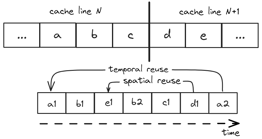
Since a unit of memory access in a modern processor is a cache line, we define two additional terms: temporal reuse happens when both use and reuse access exactly the same address and spatial reuse occurs when its use and reuse access different addresses that are located in the same cache line. Consider a sequence of memory accesses shown in Figure 8: a1,b1,e1,b2,c1,d1,a2, where locations a, b, and c occupy cache line N, and locations d and e reside on subsequent cache line N+1. In this example, the temporal reuse distance of access a2 is four, because there are four unique locations accessed between the two consecutive accesses to a, namely, b, c, d, and e. Access d1 is not a temporal reuse, however, it is a spatial reuse since we previously accessed location e, which resides on the same cache line as d. The spatial reuse distance of access d1 is two.

Figure 8. Example of temporal and spatial reuse.

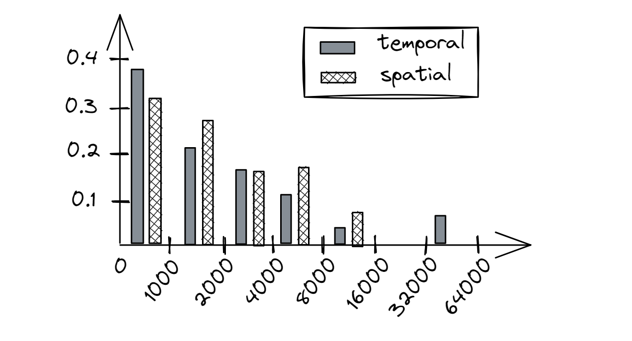
Figure 9 provides an example of a reuse distance histogram of a hypothetical program. Its X-axis is clustered in log2 bins each scaled by 1000. The Y-axis provides the rate of occurrence, i.e., how frequently we observed a certain reuse distance. Ideally, we would like to see all of the accesses in the first bin [0;1000], for both temporal and spatial reuses. For instance, for sequential access to a large array, we would see a big temporal reuse distance (bad), but a small spatial reuse distance (good). For a program that traverses a binary tree of 1000 elements (fits in L1 cache) many times, we would see relatively small temporal reuse distance (good), but big spatial reuse distance (bad). Random accesses to a large buffer represent both bad temporal and spatial locality. As a general rule, if a memory access has either a small temporal or spatial reuse distance, then it is likely to hit CPU caches. Consequently, if an access has both big temporal and big spatial reuse distances, then it is likely to miss CPU caches.

Figure 9. Example of a reuse distance histogram. X-axis is the reuse distance, Y-axis is the rate of occurrence.

Several tools were developed during the years that attempt to analyze the temporal and spatial locality of programs. Here are the three most recent tools along with their short description and current state:

• loca, a reuse distance analysis tool implemented using PIN binary-instrumentation tool. It prints reuse distance histograms for an entire program, however it can’t provide a similar breakdown for individual loads. Since it uses dynamic binary instrumentation, it incurs huge runtime (~50x) and memory (~40x) overheads, which makes the tool impractical to use in real-life applications. The tool is no longer maintained and requires some source code modifications to get it working on newer platforms. Github repo, [LocaPaper]
• RDX, utilizes hardware performance counter sampling with hardware debug registers to produce reuse-distance histograms. In contrast to loca, it incurs an order of magnitude smaller overhead while maintaining 90% accuracy. The tool is no longer maintained and there is almost no documentation on how to use the tool. [RDXpaper]
• ReuseTracker, is built upon RDX, but it extends it by taking cache-coherence and cache line invalidation effects into account. Using this tool we were able to produce meaningful results on a small program, however, it is not production quality yet and is not easy to use. Github repo, [ReuseTrackerPaper]

Aggregating reuse distances for all memory accesses in a program may be useful in some cases, but future profiling tools should also be able to provide reuse distance histograms for individual loads. Luckily, not every load/store assembly instruction has to be thoroughly analyzed. A performance engineer should first find a problematic load or store instruction using a traditional sampling approach. After that, he/she should be able to request a temporal and spatial reuse distance histogram for that particular operation. Perhaps, it should be a separate collection since it may involve a relatively large overhead.

Temporal and spatial locality analysis provides unique insights that can be used for guiding performance optimizations. However, careful implementation is not straightforward and may become tricky once we start accounting for various cache-coherence effects. Also, a large overhead may become an obstacle to integrating this feature into production profilers.