Memory Profiling Part 1. Introduction

Subscribe to my newsletter, support me on Patreon or by PayPal donation.

I would love to hear your feedback!

I wrote this blog series for the second edition of my book titled “Performance Analysis and Tuning on Modern CPUs”. It is open-sourced on Github: perf-book. The book primarily targets mainstream C and C++ developers who want to learn low-level performance engineering, but devs in other languages may also find some useful information.

After you read this write-up, let me know which parts you find useful/boring/complicated, and which parts need better explanation? Send me suggestions about the tools that I use and if you know better ones.

Tell me what you think in the comments or send me an email, which you can find here. Also, you’re welcome to write your suggestions in Github, here is the corresponding pull request.

Please keep in mind that it is an excerpt from the book, so some phrases may sound too formal.

P.S. If you’d rather read this in the form of a PDF document, you can download it here.

• Part 1: Introduction (this article).
• Part 2: Memory Usage Case Study.
• Part 3: Memory Footprint with SDE.
• Part 4: Memory Footprint Case Study.
• Part 5: Data Locality and Reuse Distances.

Memory Profiling Introduction

In this series of blog posts, you will learn how to collect high-level information about a program’s interaction with memory. This process is usually called memory profiling. Memory profiling helps you understand how an application uses memory over time and helps you build the right mental model of a program’s behavior. Here are some questions it can answer:

• What is a program’s total memory consumption and how it changes over time?
• Where and when does a program make heap allocations?
• What are the code places with the largest amount of allocated memory?
• How much memory a program accesses every second?

When developers talk about memory consumption, they implicitly mean heap usage. Heap is, in fact, the biggest memory consumer in most applications as it accommodates all dynamically allocated objects. But heap is not the only memory consumer. For completeness, let’s mention others:

• Stack: Memory used by frame stacks in an application. Each thread inside an application gets its own stack memory space. Usually, the stack size is only a few MB, and the application will crash if it exceeds the limit. The total stack memory consumption is proportional to the number of threads running in the system.
• Code: Memory that is used to store the code (instructions) of an application and its libraries. In most cases, it doesn’t contribute much to the memory consumption but there are exceptions. For example, the Clang C++ compiler and Chrome browser have large codebases and tens of MB code sections in their binaries.

Next, we will introduce the terms memory usage and memory footprint and see how to profile both.

Memory Usage and Footprint

Memory usage is frequently described by Virtual Memory Size (VSZ) and Resident Set Size (RSS). VSZ includes all memory that a process can access, e.g., stack, heap, the memory used to encode instructions of an executable, and instructions from linked shared libraries, including the memory that is swapped out to disk. On the other hand, RSS measures how much memory allocated to a process resides in RAM. Thus, RSS does not include memory that is swapped out or was never touched yet by that process. Also, RSS does not include memory from shared libraries that were not loaded to memory.

Consider an example. Process A has 200K of stack and heap allocations of which 100K resides in the main memory, the rest is swapped out or unused. It has a 500K binary, from which only 400K was touched. Process A is linked against 2500K of shared libraries and has only loaded 1000K in the main memory.

VSZ: 200K + 500K + 2500K = 3200K
RSS: 100K + 400K + 1000K = 1500K

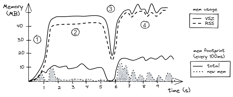
An example of visualizing the memory usage and footprint of a hypothetical program is shown in Figure 1. The intention here is not to examine statistics of a particular program, but rather to set the framework for analyzing memory profiles. Later in this chapter, we will examine a few tools that let us collect such information.

Let’s first look at the memory usage (upper two lines). As we would expect, the RSS is always less or equal to the VSZ. Looking at the chart, we can spot four phases in the program. Phase 1 is the ramp-up of the program during which it allocates its memory. Phase 2 is when the algorithm starts using this memory, notice that the memory usage stays constant. During phase 3, the program deallocates part of the memory and then allocates a slightly higher amount of memory. Phase 4 is a lot more chaotic than phase 2 with many objects allocated and deallocated. Notice, that the spikes in VSZ are not necessarily followed by corresponding spikes in RSS. That might happen when the memory was reserved by an object but never used.

Figure 1. Example of the memory usage and footprint (hypothetical scenario).

Now let’s switch to memory footprint. It defines how much memory a process touches during a period, e.g., in MB per second. In our hypothetical scenario, visualized in Figure 1, we plot memory usage per 100 milliseconds (10 times per second). The solid line tracks the number of bytes accessed during each 100 ms interval. Here, we don’t count how many times a certain memory location was accessed. That is, if a memory location was loaded twice during a 100ms interval, we count the touched memory only once. For the same reason, we cannot aggregate time intervals. For example, we know that during the phase 2, the program was touching roughly 10MB every 100ms. However, we cannot aggregate ten consecutive 100ms intervals and say that the memory footprint was 100 MB per second because the same memory location could be loaded in adjacent 100ms time intervals. It would be true only if the program never repeated memory accesses within each of 1s intervals.

The dashed line tracks the size of the unique data accessed since the start of the program. Here, we count the number of bytes accessed during each 100 ms interval that have never been touched before by the program. For the first second of the program’s lifetime, most of the accesses are unique, as we would expect. In the second phase, the algorithm starts using the allocated buffer. During the time interval from 1.3s to 1.8s, the program accesses most of the locations in the buffer, e.g., it was the first iteration of a loop in the algorithm. That’s why we see a big spike in the newly seen memory locations from 1.3s to 1.8s, but we don’t see many unique accesses after that. From the timestamp 2s up until 5s, the algorithm mostly utilizes an already-seen memory buffer and doesn’t access any new data. However, the behavior of phase 4 is different. First, during phase 4, the algorithm is more memory intensive than in phase 2 as the total memory footprint (solid line) is roughly 15 MB per 100 ms. Second, the algorithm accesses new data (dashed line) in relatively large bursts. Such bursts may be related to the allocation of new memory regions, working on them, and then deallocating them.

We will show how to obtain such charts in the following two case studies, but for now, you may wonder how this data can be used. Well, first, if we sum up unique bytes (dotted lines) accessed during every interval, we will get the total memory footprint of a program. Also, by looking at the chart, you can observe phases and correlate them with the code that is running. Ask yourself: “Does it look according to your expectations, or the workload is doing something sneaky?” You may encounter unexpected spikes in memory footprint. Memory profiling techniques that we will discuss in this series of posts do not necessarily point you to the problematic places similar to regular hotspot profiling but they certainly help you better understand the behavior of a workload. On many occasions, memory profiling helped identify a problem or served as an additional data point to support the conclusions that were made during regular profiling.

In some scenarios, memory footprint helps us estimate the pressure on the memory subsystem. For instance, if the memory footprint is small, say, 1 MB/s, and the RSS fits into the L3 cache, we might suspect that the pressure on the memory subsystem is low; remember that available memory bandwidth in modern processors is in GB/s and is getting close to 1 TB/s. On the other hand, when the memory footprint is rather large, e.g., 10 GB/s and the RSS is much bigger than the size of the L3 cache, then the workload might put significant pressure on the memory subsystem.

-> part 2