Memory Profiling Part 4. Memory Footprint Case Study

Subscribe to my newsletter, support me on Patreon or by PayPal donation.

• Part 1: Introduction.
• Part 2: Memory Usage Case Study.
• Part 3: Memory Footprint with SDE.
• Part 4: Memory Footprint Case Study (this article).
• Part 5: Data Locality and Reuse Distances.

Case Study: Memory Footprint of Four Workloads

In this case study we will use the Intel SDE tool to analyze the memory footprint of four production workloads: Blender ray tracing, Stockfish chess engine, Clang++ compilation, and AI_bench PSPNet segmentation. We hope that this study will give you an intuition of what you could expect to see in real-world applications. In part3 , we collected memory footprint per intervals of 28K instructions, which is too small for applications running hundreds of billions of instructions. So, we will measure footprint per one billion instructions.

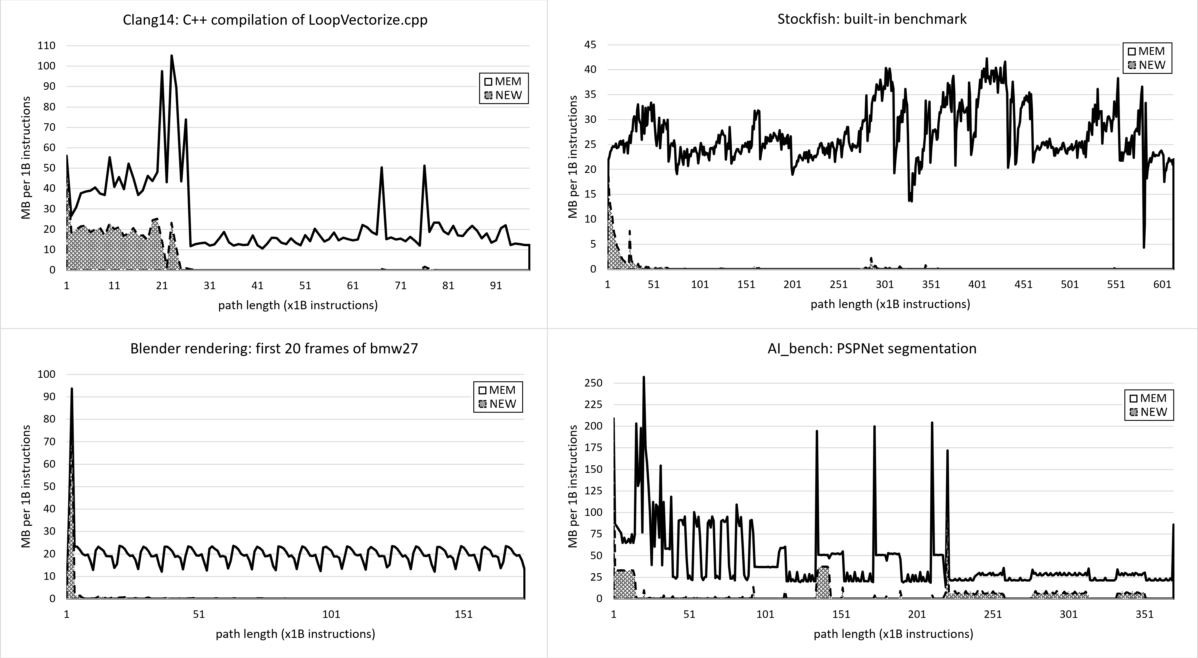
Figure 7 shows the memory footprint of four selected workloads. You can see they all have very different behavior. Clang compilation has very high memory activity at the beginning, sometimes spiking to 100MB per 1B instructions, but after that, it decreases to about 15MB per 1B instructions. Any of the spikes on the chart may be concerning to a Clang developer: are they expected? Could they be related to some memory-hungry optimization pass? Can the accessed memory locations be compacted?

Figure 7. A case study of memory footprints of four workloads. MEM - total memory accessed during 1B instructions interval. NEW - accessed memory that has not been seen before.

The Blender benchmark is very stable; we can clearly see the start and the end of each rendered frame. This enables us to focus on just a single frame, without looking at the entire 1000+ frames. The Stockfish benchmark is a lot more chaotic, probably because the chess engine crunches different positions which require different amounts of resources. Finally, the AI_bench memory footprint is very interesting as we can spot repetitive patterns. After the initial startup, there are five or six sine waves from 40B to 95B, then three regions that end with a sharp spike to 200MB, and then again three mostly flat regions hovering around 25MB per 1B instructions. All this could be actionable information that can be used to optimize the application.

There could still be some confusion about instructions as a measure of time, so let us address that. You can approximately convert the timeline from instructions to seconds if you know the IPC of the workload and the frequency at which a processor was running. For instance, at IPC=1 and processor frequency of 4GHz, 1B instructions run in 250 milliseconds, at IPC=2, 1B instructions run in 125 ms, and so on. This way, you can convert the X-axis of a memory footprint chart from instructions to seconds. But keep in mind, that it will be accurate only if the workload has a steady IPC and the frequency of the CPU doesn’t change while the workload is running.

-> part 5