Memory Profiling Part 3. Memory Footprint with SDE

Subscribe to my newsletter, support me on Patreon or by PayPal donation.

• Part 1: Introduction.
• Part 2: Memory Usage Case Study.
• Part 3: Memory Footprint with SDE (this article).
• Part 4: Memory Footprint Case Study.
• Part 5: Data Locality and Reuse Distances.

Analyzing Memory Footprint with SDE

Now let’s take a look at how we can estimate the memory footprint. In part 3, we will warm up by measuring the memory footprint of a simple program. In part 4, we will examine the memory footprint of four production workloads.

Consider a simple naive matrix multiplication code presented in the listing below on the left. The code multiplies two square 4Kx4K matrices a and b and writes the result into square 4Kx4K matrix c. Recall that to calculate one element of the result matrix c, we need to calculate the dot product of a corresponding row in the matrix a and a column in matrix b; this is what the innermost loop over k is doing.

Listing: Applying loop interchange to naive matrix multiplication code.

constexpr int N = 1024*4;                      // 4K
std::array<std::array<float, N>, N> a, b, c;   // 4K x 4K matrices
// init a, b, c
for (int i = 0; i < N; i++) {               for (int i = 0; i < N; i++) { 
  for (int j = 0; j < N; j++) {        =>     for (int k = 0; k < N; k++) {
    for (int k = 0; k < N; k++)        =>       for (int j = 0; j < N; j++) {
      c[i][j] += a[i][k] * b[k][j];               c[i][j] += a[i][k] * b[k][j];
    }                                           }
  }                                           }
}                                           }

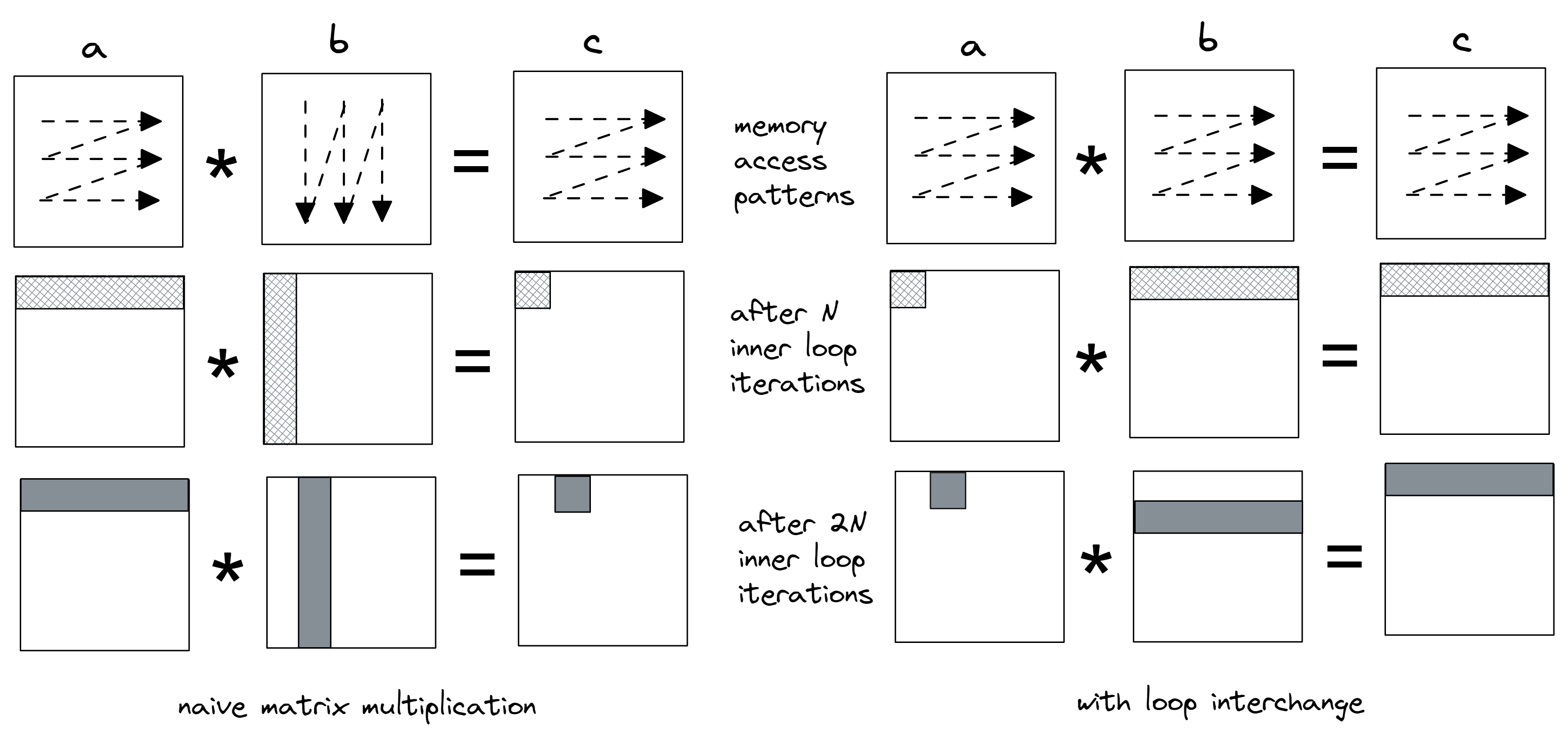
To demonstrate the memory footprint reduction, we applied a simple loop interchange transformation that swaps the loops over j and k (lines marked with =>). Once we measure the memory footprint and compare it between the two versions, it will be easy to see the difference. The visual result of the change in memory access pattern is shown in Figure 6. We went from calculating each element of matrix c one by one to calculating partial results while maintaining row-major traversal in all three matrices.

In the original code (on the left), matrix b is accessed in a column-major way, which is not cache-friendly. Look at the picture and observe the memory regions that are touched after the first N iterations of the inner loop. We calculate the dot product of row 0 in a and column 0 in b, and save it into the first element in matrix c. During the next N iterations of the inner loop, we access the same row 0 in a and column 1 in b to get the second result in matrix c.

In the transformed code on the right, the inner loop accesses just a single element in the matrix a. We multiply it by all the elements in the corresponding row in b and accumulate products into the corresponding row in c. Thus, the first N iterations of the inner loop calculate products of element 0 in a and row 0 in b and accumulate partial results in row 0 in c. Next N iterations multiply element 1 in a and row 1 in b and, again, accumulate partial results in row 0 in c.

Figure 6. Memory access pattern and cache lines touched after the first N and 2N iterations of the inner loop (images not to scale).

Let’s confirm it with Intel SDE, Software Development Emulator tool for x86-based platforms. SDE is built upon the dynamic binary instrumentation mechanism, which enables intercepting every single instruction. It comes with a huge cost. For the experiment we run, a slowdown of 100x is common.

To prevent compiler interference in our experiment, we disabled vectorization and unrolling optimizations, so that each version has only one hot loop with exactly 7 assembly instructions. We use this to uniformly compare memory footprint intervals. Instead of time intervals, we use intervals measured in machine instructions. The command line we used to collect memory footprint with SDE, along with the part of its output, is shown in the output below. Notice we use the -fp_icount 28K option which indicates measuring memory footprint for each interval of 28K instructions. This value is specifically chosen because it matches one iteration of the inner loop in “before” and “after” cases: 4K inner loop iterations * 7 instructions = 28K.

By default, SDE measures footprint in cache lines (64 bytes), but it can also measure it in memory pages (4KB on x86). We combined the output and put it side by side. Also, a few non-relevant columns were removed from the output. The first column PERIOD marks the start of a new interval of 28K instructions. The difference between each period is 28K instructions. The column LOAD tells how many cache lines were accessed by load instructions. Recall from the previous discussion, the same cache line accessed twice counts only once. Similarly, the column STORE tells how many cache lines were stored. The column CODE counts accessed cache lines that contain instructions that were executed during that period. Finally, NEW counts cache lines touched during a period, that were not seen before by the program.

Important note before we proceed: the memory footprint reported by SDE does not equal to utilized memory bandwidth. It is because it doesn’t account for whether a memory operation was served from cache or memory.

Listing: Memory footprint of naive Matmul (left) and with loop interchange (right)

$ sde64 -footprint -fp_icount 28K -- ./matrix_multiply.exe

============================= CACHE LINES =============================
PERIOD    LOAD  STORE  CODE  NEW   |   PERIOD    LOAD  STORE  CODE  NEW
-----------------------------------------------------------------------
...                                    ...
2982388   4351    1     2   4345   |   2982404   258    256    2    511
3011063   4351    1     2      0   |   3011081   258    256    2    256
3039738   4351    1     2      0   |   3039758   258    256    2    256
3068413   4351    1     2      0   |   3068435   258    256    2    256
3097088   4351    1     2      0   |   3097112   258    256    2    256
3125763   4351    1     2      0   |   3125789   258    256    2    256
3154438   4351    1     2      0   |   3154466   257    256    2    255
3183120   4352    1     2      0   |   3183150   257    256    2    256
3211802   4352    1     2      0   |   3211834   257    256    2    256
3240484   4352    1     2      0   |   3240518   257    256    2    256
3269166   4352    1     2      0   |   3269202   257    256    2    256
3297848   4352    1     2      0   |   3297886   257    256    2    256
3326530   4352    1     2      0   |   3326570   257    256    2    256
3355212   4352    1     2      0   |   3355254   257    256    2    256
3383894   4352    1     2      0   |   3383938   257    256    2    256
3412576   4352    1     2      0   |   3412622   257    256    2    256
3441258   4352    1     2   4097   |   3441306   257    256    2    257
3469940   4352    1     2      0   |   3469990   257    256    2    256
3498622   4352    1     2      0   |   3498674   257    256    2    256
...

Let’s discuss the numbers that we see in the output above. Look at the period that starts at instruction 2982388 on the left. That period corresponds to the first 4096 iterations of the inner loop in the original Matmul program. SDE reports that the algorithm has loaded 4351 cache lines during that period. Let’s do the math and see if we get the same number. The original inner loop accesses row 0 in matrix a. Remember that the size of float is 4 bytes and the size of a cache line is 64 bytes. So, for matrix a, the algorithm loads (4096 * 4 bytes) / 64 bytes = 256 cache lines. For matrix b, the algorithm accesses column 0. Every element resides on its own cache line, so for matrix b it loads 4096 cache lines. For matrix c, we accumulate all products into a single element, so 1 cache line is stored in matrix c. We calculated 4096 + 256 = 4352 cache lines loaded and 1 cache line stored. The difference in one cache line may be related to SDE starting counting 28K instruction interval not at the exact start of the first inner loop iteration. We see that there were two cache lines with instructions (CODE) accessed during that period. The seven instructions of the inner loop reside in a single cache line, but the 28K interval may also capture the middle loop, making it two cache lines in total. Lastly, since all the data that we access haven’t been seen before, all the cache lines are NEW.

Now let’s switch to the next 28K instructions period (3011063), which corresponds to the second set of 4096 iterations of the inner loop in the original Matmul program. We have the same number of LOAD, STORE, and CODE cache lines as in the previous period, which is expected. However, there are no NEW cache lines touched. Let’s understand why that happens. Look again at the Figure 6. The second set of 4096 iterations of the inner loop accesses row 0 in matrix a again. But it also accesses column 1 in matrix b, which is new, but these elements reside on the same set of cache lines as column 0, so we have already touched them in the previous 28K period. The pattern repeats through 14 subsequent periods. Each cache line contains 64 bytes / 4 bytes (size of float) = 16 elements, which explains the pattern: we fetch a new set of cache lines in matrix b every 16 iterations. The last remaining question is why we have 4097 NEW lines after the first 16 iterations of the inner loop. The answer is simple: the algorithm keeps accessing row 0 in the matrix a, so all those new cache lines come from matrix b.

For the transformed version, the memory footprint looks much more consistent with all periods having very similar numbers, except the first. In the first period, we access 1 cache line in the matrix a; (4096 * 4 bytes) / 64 bytes = 256 cache lines in b; (4096 * 4 bytes) / 64 bytes = 256 cache line are stored into c, a total of 513 lines. Again, the difference in results is related to SDE starting counting 28K instruction interval not at the exact start of the first inner loop iteration. In the second period (3011081), we access the same cache line from matrix a, a new set of 256 cache lines from matrix b, and the same set of cache lines from matrix c. Only the lines from matrix b have not been seen before, that is why the second period has NEW 256 cache lines. The period that starts with the instruction 3441306 has 257 NEW lines accessed. One additional cache line comes from accessing element a[0][17] in the matrix a, as it hasn’t been accessed before.

In the two scenarios that we explored, we confirmed our understanding of the algorithm by the SDE output. But be aware that you cannot tell whether the algorithm is cache-friendly just by looking at the output of the SDE footprint tool. In our case, we simply looked at the code and explained the numbers fairly easily. But without knowing what the algorithm is doing, it’s impossible to make the right call. Here’s why. The L1 cache in modern x86 processors can only accommodate up to ~1000 cache lines. When you look at the algorithm that accesses, say, 500 lines per 1M instructions, it may be tempting to conclude that the code must be cache-friendly, because 500 lines can easily fit into the L1 cache. But we know nothing about the nature of those accesses. If those accesses are made randomly, such code is far from being “friendly”. The output of the SDE footprint tool merely tells us how much memory was accessed, but we don’t know whether those accesses hit caches or not.

-> part 4