Benchmarking: compare measurements and check which is faster.

Contents:

• Average, Median, Minimum
• Closer look at Minimum
• So, which one to pick?
• Interestingness threshold
• Conclusion and practical advices
• Bonus: Bimodal distribution
• References

Subscribe to my newsletter, support me on Patreon or by PayPal donation.

UPD. on Jan 6th 2020 after comments from readers.

When doing performance improvements in our code, we need a way to prove that we actually made it better. Or when we commit a regular code change, we want to make sure performance did not regress. Typically, we do this by 1) measure the baseline performance, 2) measure performance of the modified program and 3) compare them with each other.

Here is the exact scenario for this article: compare performance of two different versions of the same functional program. For example, we have a program that recursively calculates Fibonacci numbers and we decided to rewrite it in an iterative fashion. Both are functionally correct and yield the same numbers. Now we need to compare two programs for performance.

It is very much recommended to get not just a single measurement, but to run the benchmark multiple times. So, we have N measurements for the baseline and N measurements for the modified version of the program. Now we need a way to compare those 2 sets of measurements to decide which one is faster.

Don’t want to scare you upfront, but it is a harder problem than you might think. Regardless, we know how to compare two scalar numbers, right? So, we can simplify this problem if we aggregate each set of measurements with a single value. Then it will boil down to just comparing 2 numbers. Easy-peasy!

If you ask any data scientist, (s)he will tell you that you should not rely on a single metric (min/mean/median, etc.). However, the classic statistical methods don’t always work well in performance world which makes the problem of automation harder. Likely manual intervention is needed in this case which makes it very time consuming. If you have nightly performance testing in place and multiple benchmarks in a suite, you can’t compare them manually every day, so automation is needed. I think that sometimes you can (and should) allow yourself to drive less accurate conclusions from the measurements in order to save your precious time.

The easiest way to automate such comparisons is by aggregating each set of measurements and pick one representative value from each. And more often than not we take… “Average, you say?”

Average, Median, Minimum

Let’s take a look at example. Suppose we have a set of 3 measurements:

{ 100s ; 120s ; 1000s }

Here is what we get if we were to visualize the measurements:

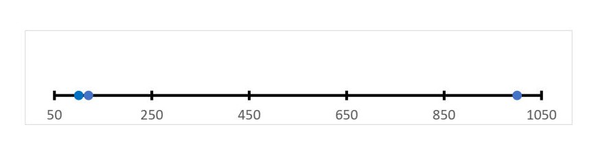
Third measurement is way off but imagine that the network got disconnected during the 3rd iteration and it took a long time to recover.

Taking average(mean) would be a bad choice in this situation. Taking median¹ would be much better. Also taking minimum would be acceptable:

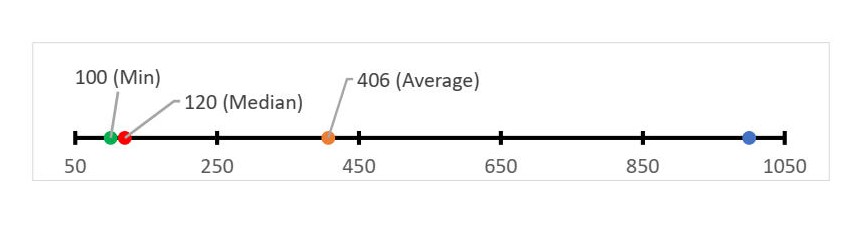
From a statistical point of view we should be collecting more samples, because the standard deviation is very high (stddev = 420s). I.e. we should be running our benchmark more times until we get more accurate and repeatable results. However, sometimes you cannot afford it. For example, some of the SPEC benchmarks run for more than 10 minutes on a modern machines. That means it takes 1 hour to produce just 3 samples: 30 minutes for each version of the program. Imagine that you have not just a single benchmark in your suite, which may make it very expensive to collect statistically sufficient data.

Let me defer explanation on why I think taking average is a bad choice and talk about minimums first. Usually they may give the BEST representative value and it is for a reason. By “representative value” I mean some value within the measurement range which will yield the most accurate comparison with the other version of a program. Mathematically speaking, we want to pick 2 values from 2 distributions such that the ratio between them would be close to the ratio between true means² from those 2 distributions.

Closer look at Minimum

Vast majority of compute-bound³ applications tend to have right-skewed distribution:

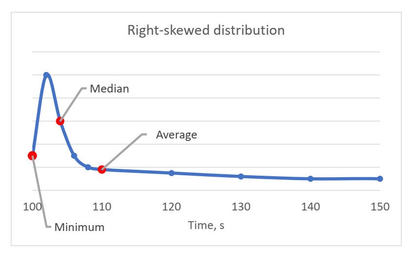
And it makes perfect sense. Imagine application runs for some time t = t1 + t2 + t3 ..., where t1 is the actual time the program needs, t2 is the time the program waited due to a missing entry in the filesystem cache, t3 is the time the program waited due to context switch by the OS, and so on. t1 is always constant in deterministic environment and is the minimum time the program needs when executed on a certain platform. But because there is a lot of non-determinism in modern systems, we have a lot of variables in the equation. Consider the situation when the application we measure, downloads some file from the internet⁴. It may be very quickly if we were lucky or very slow otherwise.

If you look at the chart, you may drive certain guesses from it. Sometimes we were lucky enough to run very fast (minimum). Those were few iterations where no cache misses happened, the process was never context-switched out, etc. But more often, we were not so lucky, and we had some performance “road blocks” on our way (spike around 102 sec). And also, there were iterations when we had some major performance problems (measurements greater than 110 sec), like, for example, we ran out of memory and OS performed memory swapping to the disk.

When we compare performance of two versions of the program, we really want to compare their t1 components and throw away all the other variables. Minimum value from 2 sets of measurements could yield the most accurate comparison in this situation.

Now, going back to our first example… Remember I wrote that taking average is a bad choice? But why? Mathematically, it is the best choice the one could make if not considering that there could be… Outliers. We know the underlying nature of the environment we are working in and it suggests us that the rightmost sample (1000s) is likely to be an outlier. The issue with the average is that it accounts for outliers which we should be removing first. Minimum is free from taking into account right hand side outliers, which allows to have smaller number of iterations. Median is resistant to both left- and right-hand side outliers, but sometimes does not give the most accurate comparisons.

That said, on practice minimum works well for right-skewed distributions, e.g. compute-bound workloads. However, there are cases when minimum can also be a bad choice. For example:

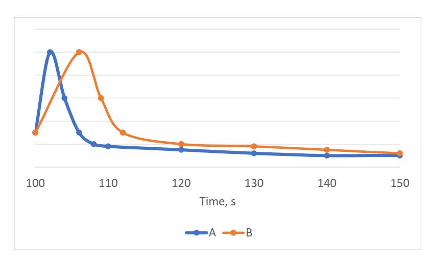
In this scenario both A and B versions have the same minimum value, but we clearly can see that usually A is faster. Dah! I know, I might confused you at this point and you want to ask…

So, which one to pick?

It turns out that there is no right or wrong answer. There is no easy way to compare distributions. And it is not always easy to do. We can only hypothesize that some version of a program is faster than the other, because the measurement set is endless. We can always produce additional sample which could be way faster than all the previous. We can only say that we think the version A is faster than version B with some probability P. You see, it gets complicated really quickly…

So, what do you do? You look at the distribution.⁵

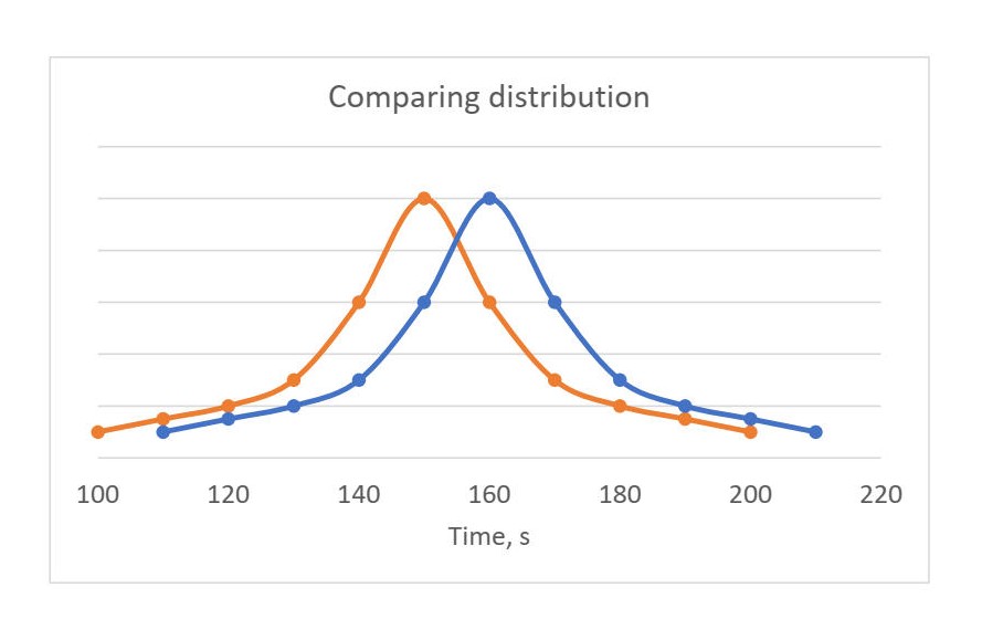
By looking at those diagrams we can make conclusions with somewhat high level of confidence. On the left chart we can say that version of the program that corresponds to orange line is faster than the blue one.

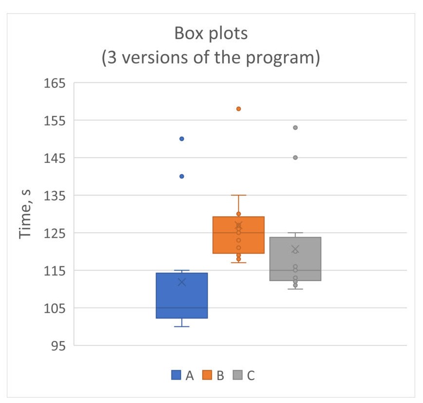
Box plots are widely used for comparing distributions of many benchmarks on a single chart. We can say that version A is faster than version C and C is faster than B. Usually scientific papers tend to present their results with box plots and let readers drive their own conclusion out of them.

That’s why it is essential to know the distribution of the benchmark you are working with. If you know characteristics (distribution) for your benchmark, you can do the visualization once, decide on what you will choose as a “representative value” and then automate it. For example, I work exclusively with compute bound workloads, so I know their distribution is right-skewed, in which case it’s okay to take the minimum or median.

Interestingness threshold

When comparing two versions of the same program, some fluctuation in performance is inevitable. Imagine, we have a nightly performance testing in place. And quite often you will see performance variations as developers commit their changes. Sometimes small performance degradations can arise even without code changes due to HW instability, I/O, environment, etc. Sometimes even a harmless code change can trigger performance variation of your benchmark. Example of such HW effect can be found in my earlier article Code placement issues.

Since usually we cannot do much about instability described above, it would be good to filter somehow the noise from the real regressions resulted from a bad code change. The last thing we want is to be bothered with everyday performance changes of 0.5% up or down. Understanding whether regression comes from a bad code change or from other sources can be quite time consuming, especially if it a small regression (<2%).

To deal with such kind of issues we need to define some threshold which we will use to filter small performance variation. For example, if we set the interestingness threshold to 2%, it means that every performance change below it will be considered as noise and can be ignored. Keep in mind, that by using such a criterion, sometimes you can ignore the real performance regressions. This is a business decision to make and is a trade-off. On the one hand you want to save your time and avoid analyzing small regressions that often are just noise. On the other hand, you might miss the bad code change.

The actual value of this threshold usually depends on 1) how much you care about performance regressions/improvements and 2) how flaky your benchmark is. For compute bound workloads I see people set their threshold in the range from 2% to 5%.

Be sure to track absolute numbers as well, not just ratios. E.g. if you have 4 consecutive 1.5% regressions, they will all be filtered by the interestingness threshold, but they will sum up to 6% over 4 days. You don’t want to skip such long-term degradation, so make sure you track the absolute numbers from time to time to see the trend in which performance of your benchmark is going.

Conclusion and practical advices

Below are the practical advices. They may not work for every possible scenario, but I hope will work well in practice.

1. No single metric is perfect.
2. If you can afford rich collection of samples (at least 30) it’s okay to compare means (averages) but only if the standard error is small. You can also adjust the number of iterations dynamically by checking standard error after each collected sample. I.e. you collect samples until you get standard error lie in a certain range.
3. If you have a small number of benchmark iterations consider taking minimum or median, because the mean can be spoiled by outliers. Alternatively, you can go through the process of removing outliers, which I will not discuss in this article. After that you can again consider comparing means. However, there are cases when you cannot remove outliers. For example, if you are benchmarking latency of a web service request, you might care a lot about outliers if you have time limits for processing each request.
4. To be on a safe side, plot the distributions and let the readers drive their own conclusions. If you decide to go without automation, likely box/violin plots are your best friends here. Alternatively you can compare distributions by representing them with at least 3 numbers: { Q1; median ; Q3 }.
5. Define the interestingness threshold for your measurements.

Bonus: Bimodal distribution

What if you visualized distribution of performance measurements for your benchmark and see something like this?

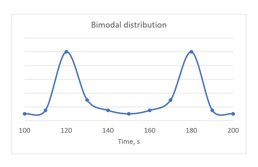
If you encountered bimodal distribution, probably there is something wrong with the benchmark. It actually means that you have 2 different types of behavior that occur with equal probability. Consider this situation when it might happen: 1) you want to make 100 runs for the benchmark, 2) first 50 iterations ran fast, 3) starting from iteration #51 someone logged in and started his own experiments which sucked computational resources from your benchmark process.

What we want to do in this situation is to isolate those 2 behaviors and test them separately.

References

1. I gained a lot of information for this article from Andrey Akinshin’s book “Pro .NET Benchmarking”⁶.
2. I also find the following article very interesting: “Benchmarking: minimum vs average”.