Subscribe to my newsletter, support me on Patreon, Github, or by PayPal donation.
I would love to hear your feedback!
I wrote this blog series for the second edition of my book titled “Performance Analysis and Tuning on Modern CPUs”. It is open-sourced on Github: perf-book. The book primarily targets mainstream C and C++ developers who want to learn low-level performance engineering, but devs in other languages may also find a lot of useful information.
After you finish, let me know which parts you find useful/boring/complicated, which parts need better explanation, etc. Write a comment or send me an email, which you can find here.
Please keep in mind that it is an excerpt from the book, so some phrases may sound too formal. Also, in the original chapter, there is a preface to this content, where I talk about Amdahl’s law, Universal Scalability Law, parallel efficiency metrics, etc. But I’m sure you guys don’t need that. :)
Estimated reading time: 25 mins. TLDR; jump straight to the summary.
- Part 1: Introduction (this article).
- Part 2: Blender and Clang.
- Part 3: Zstandard.
- Part 4: CloverLeaf and CPython.
- Part 5: Summary.
Thread Count Scaling Case Study
Thread count scaling is perhaps the most valuable analysis you can perform on a multithreaded application. It shows how well the application can utilize modern multicore systems. As you will see, there is a ton of information you can learn along the way. Without further introduction, let’s get started.
In this case study, we will analyze the thread count scaling of the following benchmarks, some of which should be already familiar to you from the previous chapters:
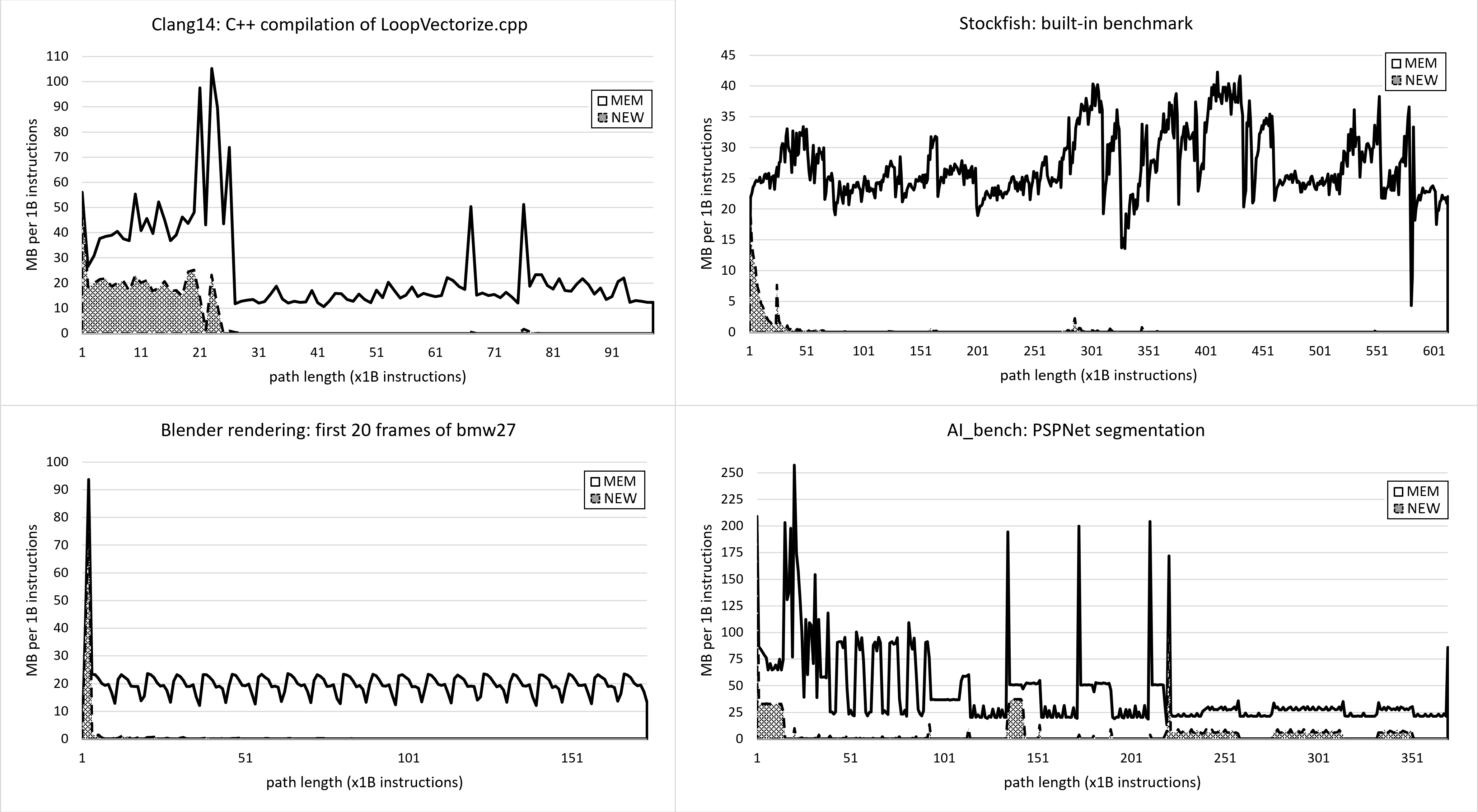
- Blender 3.4, an open-source 3D creation and modeling software project. This test is of Blender’s Cycles performance with the BMW27 blend file. Command line:
./blender -b bmw27_cpu.blend -noaudio --enable-autoexec -o output.test -x 1 -F JPEG -f 1 -t N, whereNis the number of threads. - Clang 17 self-build, this test uses clang 17 to build the clang 17 compiler from sources. Command line:
ninja -jN clang, whereNis the number of threads. - Zstandard v1.5.5, a fast lossless compression algorithm. A dataset used for compression: silesia.tar. Command line:
./zstd -TN -3 -f -- silesia.tar, whereNis the number of compression worker threads. - CloverLeaf 2018, a Lagrangian-Eulerian hydrodynamics benchmark. This test uses the input file
clover_bm.in. Command line:export OMP_NUM_THREADS=N; ./clover_leaf, whereNis the number of threads. - CPython 3.12, a reference implementation of the Python programming language. We run a simple multithreaded binary search script written in Python, which searches
10'000random numbers (needles) in a sorted list of1'000'000elements (haystack). Command line:./python3 binary_search.py N, whereNis the number of threads. Needles are divided equally between threads.
The benchmarks were executed on a machine with the configuration shown below:
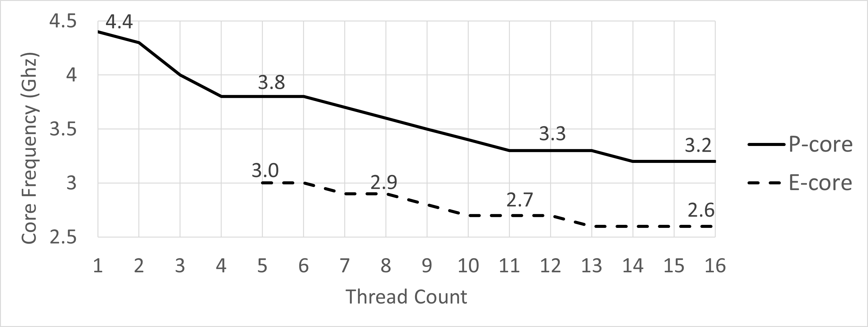
- 12th Gen Alderlake Intel(R) Core(TM) i7-1260P CPU @ 2.10GHz (4.70GHz Turbo), 4P+8E cores, 18MB L3-cache.
- 16 GB RAM, DDR4 @ 2400 MT/s.
- Clang 15 compiler with the following options:
-O3 -march=core-avx2. - 256GB NVMe PCIe M.2 SSD.
- 64-bit Ubuntu 22.04.1 LTS (Jammy Jellyfish, Linux kernel 6.5).
This is clearly not the top-of-the-line hardware setup, but rather a mainstream computer, not necessarily designed to handle media, developer, or HPC workloads. However, for our case study, it is an excellent platform to demonstrate the various effects of thread count scaling. Because of the limited resources, applications start to hit performance roadblocks even with a small number of threads. Keep in mind, that on better hardware, the scaling results will be different.
Our processor has four P-cores and eight E-cores. P-cores are SMT-enabled, which means the total number of threads on this platform is sixteen. By default, the Linux scheduler will first try to use idle physical P-cores. The first four threads will utilize four threads on four idle P-cores. When they are fully utilized, it will start to schedule threads on E-cores. So, the next eight threads will be scheduled on eight E-cores. Finally, the remaining four threads will be scheduled on the 4 sibling SMT threads of P-cores. We’ve also run the benchmarks while affinitizing threads using the aforementioned scheme, except Zstd and CPython. Running without affinity does a better job of representing real-world scenarios, however, thread affinity makes thread count scaling analysis cleaner. Since performance numbers were very similar, in this case study we present the results when thread affinity is used.
The benchmarks do a fixed amount of work. The number of retired instructions is almost identical regardless of the thread count. In all of them, the largest portion of an algorithm is implemented using a divide-and-conquer paradigm, where work is split into equal parts, and each part can be processed independently. In theory, this allows applications to scale well with the number of cores. However, in practice, the scaling is often far from optimal.
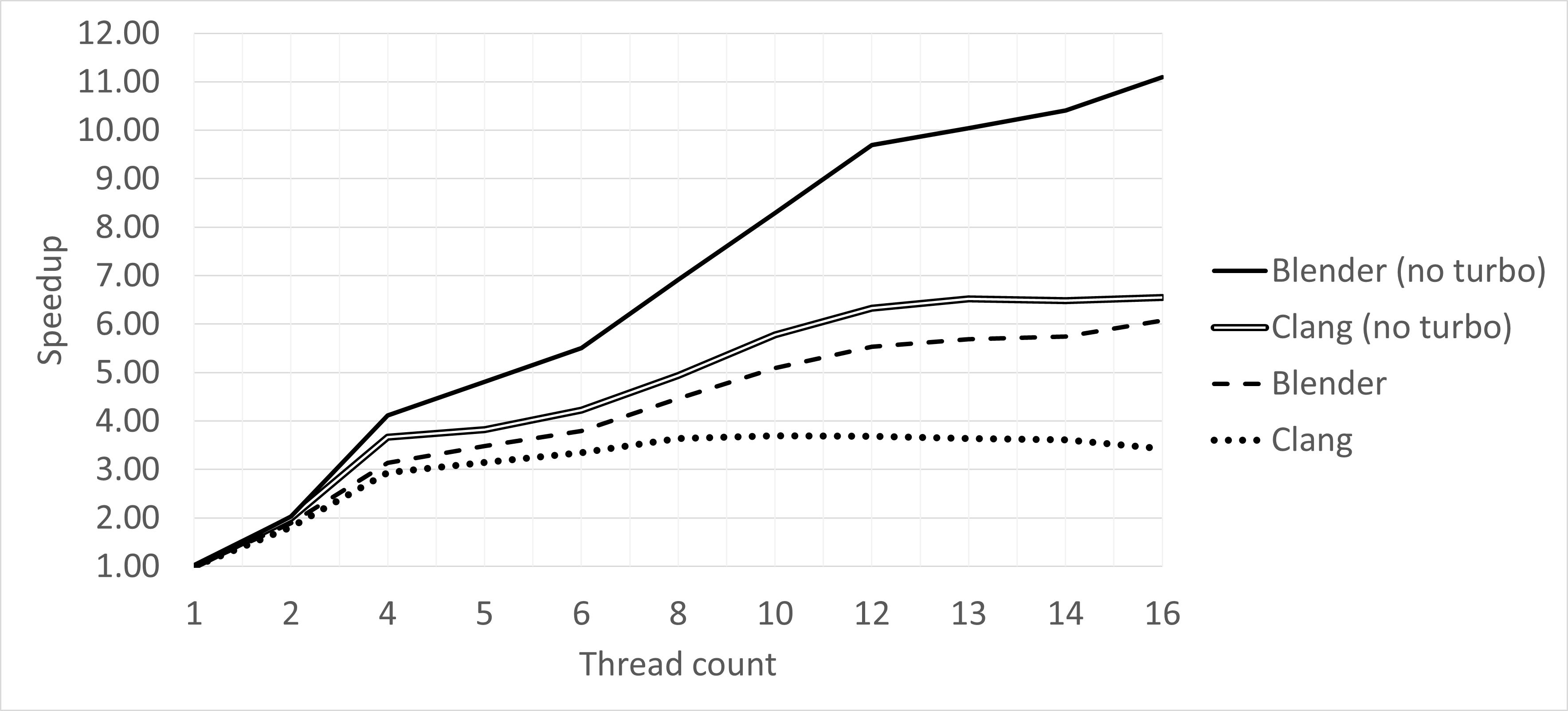
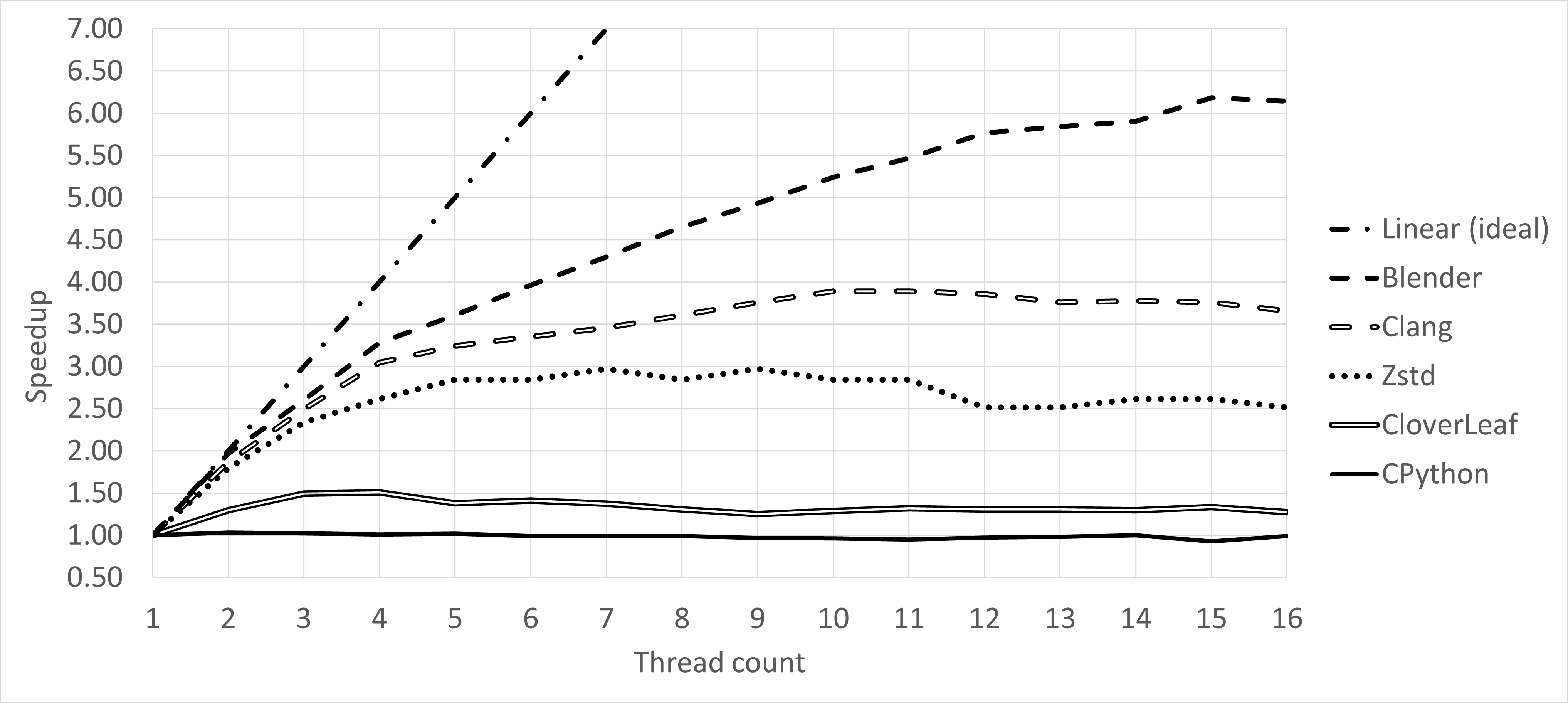
Figure 1 shows the thread count scalability of the selected benchmarks. The x-axis represents the number of threads, and the y-axis shows the speedup relative to the single-threaded execution. The speedup is calculated as the execution time of the single-threaded execution divided by the execution time of the multi-threaded execution. The higher the speedup, the better the application scales with the number of threads.
I suggest to open this image in a separate tab as we will get back to it several times.
 |
|---|
| Figure 1. Thread Count Scalability chart for five selected benchmarks. (clickable) |
As you can see, most of them are very far from the linear scaling, which is quite disappointing. The benchmark with the best scaling in this case study, Blender, achieves only 6x speedup while using 16x threads. CPython, for example, enjoys no thread count scaling at all. Performance of Clang and Zstd suddenly degrades when the number of threads goes beyond 11. To understand this and other issues, let’s dive into the details of each benchmark.
-> part 2